Обеспеченность сервисами

get_service_provision распределяет спрос зданий между сервисами с ограниченной вместимостью по матрице стоимостей пути и нормативному порогу. Этот ноутбук

1. рассчитывает обеспеченность с порогом 10 минут по заранее рассчитанной интермодальной матрице времени в пути;

2. строит карты показателя обеспеченности и нагрузки сервисов;

3. удаляет связи длиннее 8 минут функцией recalculate_links и обрезает результат по части территории;

4. повторяет расчёт с разреженной матрицей pandas.

Матрица в examples_data/matrix_time.parquet рассчитана с IduEdu (calculate_od_matrix); недостижимые пары равны inf.

Последний раздел, Своя территория, показывает, что заменить, чтобы получить такие же картинки для другой территории.

# !pip install objectnat pyarrow matplotlib

import geopandas as gpd
import matplotlib.pyplot as plt
import numpy as np
import pandas as pd

from objectnat import (
    clip_provision,
    get_provision_buildings,
    get_provision_links,
    get_provision_services,
    get_service_provision,
    recalculate_links,
)

buildings = gpd.read_parquet("examples_data/buildings.parquet")
services = gpd.read_parquet("examples_data/services.parquet")
matrix = pd.read_parquet("examples_data/matrix_time.parquet")  # minutes, rows: buildings, columns: services
print(f"{len(buildings)} buildings (demand {buildings['demand'].sum()}), "
      f"{len(services)} services (capacity {services['capacity'].sum()}), matrix {matrix.shape}")

4101 buildings (demand 29596), 36 services (capacity 31142), matrix (4101, 36)

1. Обеспеченность в пределах 10 минут

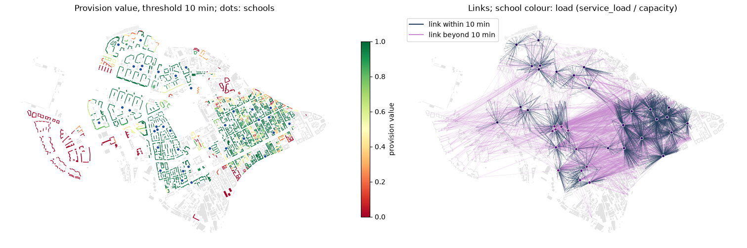
Результат — ProvisionResult: разреженная матрица flow распределённого спроса и таблицы demand_rows и capacity_rows. Фиксированный seed делает распределение воспроизводимым.

result = get_service_provision(buildings=buildings, services=services, distance_matrix=matrix, threshold=10, seed=0)
# the result brings its own demand/capacity columns, so the input ones are dropped before joining
buildings_prov = get_provision_buildings(buildings.drop(columns="demand"), result)
services_prov = get_provision_services(services.drop(columns="capacity"), result)
links = get_provision_links(buildings, services, result)

demand = result.demand_rows
print(f"supplied within 10 min: {demand['supplied_demands_within'].sum() / demand['demand'].sum():.1%}, "
      f"beyond: {demand['supplied_demands_without'].sum() / demand['demand'].sum():.1%}, "
      f"left: {demand['demand_left'].sum() / demand['demand'].sum():.1%}")
result.capacity_rows.describe().round(1)

supplied within 10 min: 61.7%, beyond: 33.4%, left: 4.9%

	capacity	capacity_left	carried_capacity_within	carried_capacity_without	service_load
count	36.0	36.0	36.0	36.0	36.0
mean	865.1	83.3	507.0	274.7	781.8
std	487.1	110.6	319.9	320.0	434.1
min	120.0	0.0	61.0	2.0	100.0
25%	550.8	13.8	242.5	42.2	457.0
50%	960.0	36.0	493.0	185.0	805.5
75%	1200.0	113.0	725.2	398.0	1138.2
max	2161.0	457.0	1145.0	1402.0	1756.0

2. Карты

provision_value — доля спроса здания, удовлетворённая сервисами в пределах порога; service_load — суммарный спрос, распределённый на сервис.

from matplotlib.lines import Line2D


def school_markers(ax, schools, color="#1f4e9c"):
    """Schools as small dots, so that the buildings around them stay visible."""
    schools.plot(ax=ax, marker="o", markersize=18, color=color, edgecolor="white", linewidth=0.6, zorder=5)


living = buildings_prov[buildings_prov["demand"] > 0]
fig, axs = plt.subplots(1, 2, figsize=(15, 6), constrained_layout=True)
ax = axs[0]
buildings_prov[buildings_prov["demand"] <= 0].plot(ax=ax, color="#e3e3e3", linewidth=0)
living.plot(ax=ax, column="provision_value", cmap="RdYlGn", vmin=0, vmax=1, legend=True,
            legend_kwds={"label": "provision value", "shrink": 0.6})
school_markers(ax, services_prov)
ax.set_title("Provision value, threshold 10 min; dots: schools")
ax = axs[1]
buildings.plot(ax=ax, color="#e3e3e3", linewidth=0)
within = links["distance"] <= 10
links[~within].plot(ax=ax, color="#c98bd0", linewidth=0.3, alpha=0.35)
links[within].plot(ax=ax, color="#26415e", linewidth=0.4, alpha=0.6)
load_share = (services_prov["service_load"] / services_prov["capacity"]).clip(0, 1)
school_markers(ax, services_prov, color=plt.get_cmap("magma_r")(0.15 + 0.7 * load_share))
ax.legend(handles=[Line2D([], [], color="#26415e", label="link within 10 min"),
                   Line2D([], [], color="#c98bd0", label="link beyond 10 min")], loc="upper left")
ax.set_title("Links; school colour: load (service_load / capacity)")
for ax in axs:
    ax.set_axis_off()
plt.show()

3. Меньший порог и обрезка

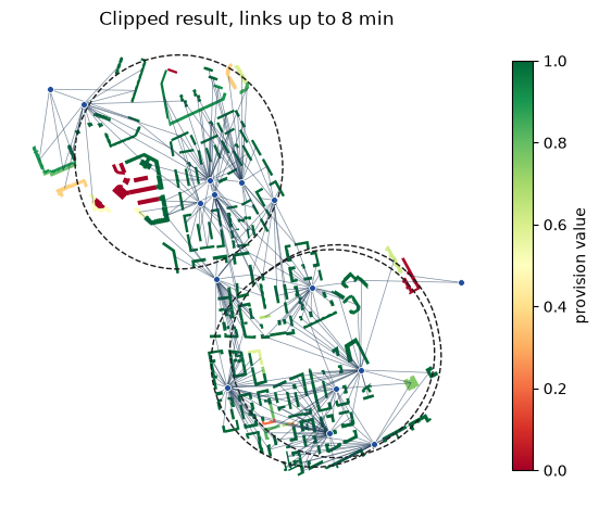
recalculate_links удаляет потоки со стоимостью больше new_max_dist и пересчитывает показатели; удалённый спрос не перераспределяется. clip_provision оставляет здания, пересекающие зону, их связи и сервисы, которыми они пользуются.

result_8 = recalculate_links(result, new_max_dist=8)
removed = result.demand_rows["demand_left"].sum(), result_8.demand_rows["demand_left"].sum()
print(f"unsupplied demand: {removed[0]} with all links, {removed[1]} after removing links longer than 8 min")

buildings_8 = get_provision_buildings(buildings.drop(columns="demand"), result_8)
services_8 = get_provision_services(services.drop(columns="capacity"), result_8)
links_8 = get_provision_links(buildings, services, result_8)

zone = buildings.iloc[500:503][["geometry"]].copy()
zone["geometry"] = zone.buffer(500)
b_clip, s_clip, l_clip = clip_provision(buildings_8, services_8, links_8, selection_zone=zone)
print(len(b_clip), "buildings,", len(s_clip), "services,", len(l_clip), "links in the zone")

unsupplied demand: 1453 with all links, 13115 after removing links longer than 8 min
449 buildings, 15 services, 363 links in the zone

fig, ax = plt.subplots(figsize=(7, 7))
zone.boundary.plot(ax=ax, color="#1a1a1a", linewidth=1, linestyle="--")
b_clip[b_clip["demand"] > 0].plot(ax=ax, column="provision_value", cmap="RdYlGn", vmin=0, vmax=1, legend=True,
                                  legend_kwds={"label": "provision value", "shrink": 0.7})
l_clip.plot(ax=ax, color="#26415e", linewidth=0.5, alpha=0.6)
school_markers(ax, s_clip)
ax.set_title("Clipped result, links up to 8 min")
ax.set_axis_off()
plt.show()

4. Разреженные матрицы

На больших территориях большинство пар здание–сервис недостижимы при любой разумной стоимости. Разреженный DataFrame pandas с NaN (или inf) в качестве заполнителя хранит только достижимые пары; get_service_provision читает его поэлементно без уплотнения. Такую матрицу возвращает od_matrix из IduEdu.

В распределении участвуют только пары со стоимостью до 3 * threshold. Поэтому при пороге 5 минут пары дальше 15 минут можно отбросить без изменения результата:

sparse = matrix.where(matrix <= 15).astype(pd.SparseDtype("float64", np.nan))
print(f"dense: {matrix.memory_usage().sum() / 1e6:.2f} MB, sparse (pairs within 15 min): "
      f"{sparse.memory_usage().sum() / 1e6:.2f} MB, density {sparse.sparse.density:.1%}")

dense_5 = get_service_provision(buildings=buildings, services=services, distance_matrix=matrix, threshold=5, seed=0)
sparse_5 = get_service_provision(buildings=buildings, services=services, distance_matrix=sparse, threshold=5, seed=0)
allocation = ["demand_left", "supplied_demands_within", "supplied_demands_without", "avg_dist", "provision_value"]
same = dense_5.demand_rows[allocation].fillna(-1).equals(sparse_5.demand_rows[allocation].fillna(-1))
print("same allocation with the dense and the sparse matrix:", same)
# min_dist is read from the matrix itself: NaN where the nearest service is beyond the 15-minute cut
print("buildings whose nearest service is beyond 15 min:", int(sparse_5.demand_rows["min_dist"].isna().sum()))

dense: 1.03 MB, sparse (pairs within 15 min): 0.31 MB, density 17.4%
same allocation with the dense and the sparse matrix: True
buildings whose nearest service is beyond 15 min: 243

5. Своя территория

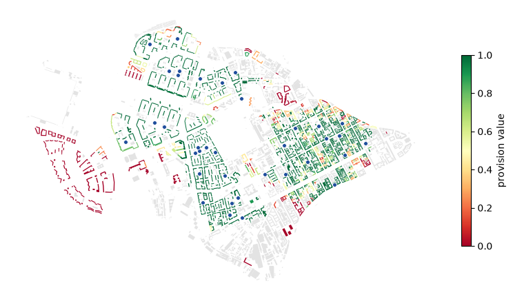
Здания со столбцом спроса, сервисы со столбцом вместимости и стоимости пути между ними (calculate_od_matrix строит матрицу для любой территории). Обеспеченность присоединяется к зданиям: нарисуйте её в matplotlib, посмотрите на веб-карте или сохраните для ГИС через to_file.

my_buildings, my_services, my_matrix = buildings, services, matrix  # matrix rows and columns: their indices

my_result = get_service_provision(
    buildings=my_buildings, services=my_services, distance_matrix=my_matrix, threshold=10, seed=0
)
my_prov = get_provision_buildings(my_buildings.drop(columns="demand"), my_result)
my_schools = get_provision_services(my_services.drop(columns="capacity"), my_result)

fig, ax = plt.subplots(figsize=(10, 6))
my_prov[my_prov["demand"] <= 0].plot(ax=ax, color="#e3e3e3", linewidth=0)
my_prov[my_prov["demand"] > 0].plot(ax=ax, column="provision_value", cmap="RdYlGn", vmin=0, vmax=1, legend=True,
                                    legend_kwds={"label": "provision value", "shrink": 0.6})
school_markers(ax, my_schools)
ax.set_axis_off()
plt.show()
# my_prov.to_file("my_provision.gpkg")  # for GIS

import folium

# a light copy for the web map: the column shown, outlines simplified by 1 m, coordinates rounded to about 10 cm
living = my_prov.loc[my_prov["demand"] > 0, ["provision_value", "geometry"]]
light = living.to_crs(living.estimate_utm_crs())
light["geometry"] = light.simplify(1.0)
light = light.to_crs(4326)
light["geometry"] = light.geometry.set_precision(1e-6)
light.explore(column="provision_value", cmap="RdYlGn", vmin=0, vmax=1, 
              tiles=folium.TileLayer("Esri.WorldGrayCanvas", max_zoom=19, max_native_zoom=16))  # light grey base map

Make this Notebook Trusted to load map: File -> Trust Notebook