Insolation: sun hours on the ground and on facades

This notebook computes hours of direct sunlight among buildings of known height with get_insolation (ground receivers) and get_facade_insolation (facade points per floor):

1. sun hours for a single day (equinox and summer solstice) as rasters (rasterize);

2. a period (22 April – 22 August) with the longest continuous sunlit period on the worst day;

3. the effect of terrain given as an array, and the raster on a web map (Raster.explore);

4. facade insolation per floor and a check against a continuous-insolation norm.

The example buildings (Vasilyevsky Island, Saint Petersburg, 59.96° N) have a storeys_count column; heights are storeys × 3 m. The method is described on the insolation page.

The last section, Your own area, shows what to replace to get the same pictures for another territory.

# !pip install objectnat pyarrow matplotlib

import geopandas as gpd

buildings = gpd.read_parquet("examples_data/buildings.parquet")  # EPSG:32636 (UTM 36N), metres
# 0 storeys means "unknown" in this dataset; such buildings get default_height below
buildings["storeys_count"] = buildings["storeys_count"].where(buildings["storeys_count"] > 0)
HEIGHTS = dict(height_column=None, storeys_column="storeys_count", storey_height=3.0, default_height=3.0)
buildings[["storeys_count", "geometry"]].describe()

	storeys_count
count	4100.000000
mean	3.243902
std	3.430774
min	1.000000
25%	1.000000
50%	1.000000
75%	5.000000
max	24.000000

import matplotlib.pyplot as plt
import numpy as np
from mpl_toolkits.axes_grid1.anchored_artists import AnchoredSizeBar


def map_extent(ax, bounds, bar=100, outline=True):
    """Show `bounds` (x0, y0, x1, y1 in metres) without coordinate axes, with a scale bar and the area outline."""
    x0, y0, x1, y1 = bounds
    pad = 0.012 * max(x1 - x0, y1 - y0)
    ax.set_xlim(x0 - pad, x1 + pad)
    ax.set_ylim(y0 - pad, y1 + pad)
    ax.set_aspect("equal")
    ax.set_axis_off()
    if outline:
        ax.plot([x0, x1, x1, x0, x0], [y0, y0, y1, y1, y0], color="#3d3d3d", linewidth=1, zorder=8)
    scale = AnchoredSizeBar(ax.transData, bar, f"{bar:g} m", loc="lower right", pad=0.4, sep=4, size_vertical=bar / 40)
    scale.patch.set(facecolor="white", edgecolor="none", alpha=0.85)
    ax.add_artist(scale)

1. Study area

A 500 × 400 m residential area with courtyards. All buildings within 300 m of it are passed to the functions, because buildings outside the area also cast shadows into it.

import shapely

from objectnat import get_facade_insolation, get_insolation

area = shapely.box(344750, 6649850, 345250, 6650250)  # in the CRS of the buildings
scene = buildings[buildings.intersects(area.buffer(300))]
shown = scene.clip(area.buffer(1))
print(f"{len(scene)} buildings in the scene, {len(shown)} in the area")

171 buildings in the scene, 50 in the area

2. One day

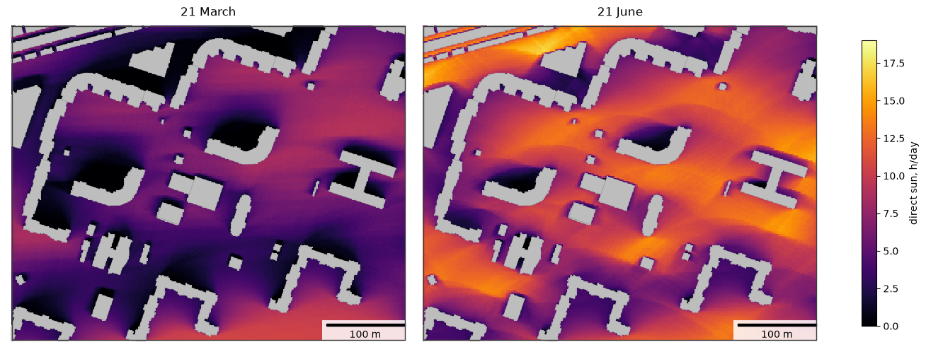
date is a single day. Receivers are placed every grid_step metres outside footprints, and the sun position is sampled every time_step_min minutes. The result is the receiver points with sun_hours (0 for ground with no direct sun at all); attrs contain the simulated days, the day length and the grid. rasterize turns a column into a Raster on the grid of the calculation, whatever CRS the receivers are in, and plot draws it with matplotlib.

import time

import pandas as pd

days = {"2026-03-21": "21 March", "2026-06-21": "21 June"}
suns = {}
for day in days:
    start = time.perf_counter()
    suns[day] = get_insolation(scene, day, area=area, grid_step=2, time_step_min=10, **HEIGHTS)
    print(f"{day}: {time.perf_counter() - start:.1f} s, day length {suns[day].attrs['day_length_hours']:.1f} h")

pd.DataFrame({title: suns[day]["sun_hours"].describe() for day, title in days.items()}).round(2)

2026-03-21: 0.2 s, day length 12.2 h

2026-06-21: 0.2 s, day length 18.7 h

	21 March	21 June
count	41207.00	41207.00
mean	4.60	9.03
std	2.79	3.21
min	0.00	0.00
25%	2.50	6.67
50%	4.50	9.50
75%	6.67	11.67
max	10.83	17.17

from objectnat import rasterize

fig, axs = plt.subplots(1, 2, figsize=(13, 5.2), constrained_layout=True)
for ax, (day, title) in zip(axs, days.items()):
    gpd.GeoSeries([area]).plot(ax=ax, color="#bdbdbd", zorder=0)  # cells without a receiver lie under buildings
    im = rasterize(suns[day], "sun_hours").plot(ax=ax, cmap="inferno", vmin=0, vmax=19)
    shown.plot(ax=ax, color="#bdbdbd", edgecolor="#8c8c8c", linewidth=0.3)
    map_extent(ax, area.bounds)
    ax.set_title(title)
fig.colorbar(im, ax=axs, shrink=0.8, label="direct sun, h/day")
plt.show()

3. A period and the worst day

date=(start, end) simulates every day_step-th day of the period and its last day. The receiver points have sun_hours (mean over the simulated days), min_sun_hours (worst day) and max_continuous_hours (longest continuous sunlit period on the worst day), for which insolation norms usually set a minimum.

receivers = get_insolation(
    scene, ("2026-04-22", "2026-08-22"), area=area, grid_step=2, day_step=7, **HEIGHTS
)
print(len(receivers.attrs["days"]), "simulated days:", receivers.attrs["days"][0], "...", receivers.attrs["days"][-1])
receivers[["sun_hours", "min_sun_hours", "max_continuous_hours"]].describe().round(2)

19 simulated days: 2026-04-22 ... 2026-08-22

	sun_hours	min_sun_hours	max_continuous_hours
count	41207.00	41207.00	41207.00
mean	8.11	6.59	5.65
std	3.04	2.96	2.89
min	0.00	0.00	0.00
25%	5.93	4.33	3.33
50%	8.59	7.00	5.50
75%	10.70	9.17	8.17
max	14.32	12.67	12.67

Both maps share one colour scale.

fig, axs = plt.subplots(1, 2, figsize=(13, 5.2), constrained_layout=True)
for ax, col, title in [
    (axs[0], "sun_hours", "22 April – 22 August, mean"),
    (axs[1], "max_continuous_hours", "22 April – 22 August, longest continuous sunlit period on the worst day"),
]:
    gpd.GeoSeries([area]).plot(ax=ax, color="#bdbdbd", zorder=0)  # cells without a receiver lie under buildings
    im = rasterize(receivers, col).plot(ax=ax, cmap="inferno", vmin=0, vmax=14)
    shown.plot(ax=ax, color="#bdbdbd", edgecolor="#8c8c8c", linewidth=0.3)
    map_extent(ax, area.bounds)
    ax.set_title(title)
fig.colorbar(im, ax=axs, shrink=0.8, label="direct sun, h/day")
plt.show()

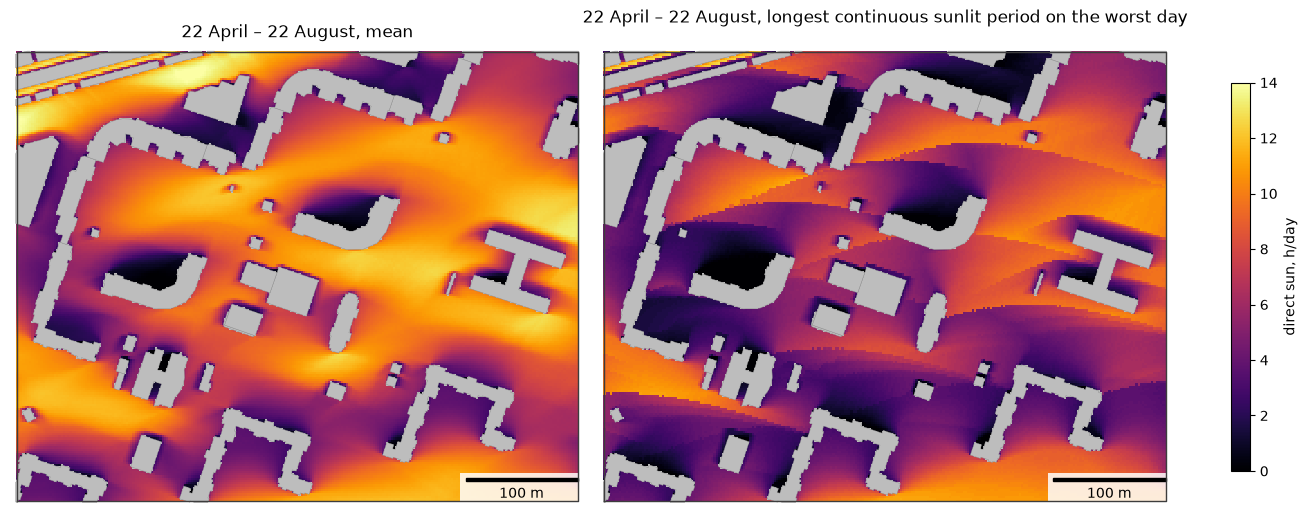
Share of the open ground in the area that receives at least 3 h of continuous sun on every simulated day:

share = (receivers["max_continuous_hours"] >= 3).mean()
print(f"{share:.0%} of the receivers")

81% of the receivers

4. Terrain

Terrain can be a GeoDataFrame of polygons with heights (rasterized with terrain_cell cells), a GeoTIFF path or a (heights, transform, crs) tuple; a Raster is such a tuple too. Here a synthetic ridge 50 m high runs west–east with its crest 50 m south of the area, given as an array with 5 m cells. Buildings stand on the terrain and receivers are placed on it, so a hill under the area itself changes little: what matters is terrain that rises above the line to the sun, here the ridge between the area and the low equinox sun.

from matplotlib import colors as mcolors

cell = 5.0
x0, y0, x1, y1 = area.buffer(400).bounds
cols, rows = int((x1 - x0) / cell), int((y1 - y0) / cell)
ys = y1 - (np.arange(rows) + 0.5) * cell  # row 0 is the northern edge
crest = area.bounds[1] - 50
ridge = 50.0 * np.exp(-((ys - crest) ** 2) / (2 * 30.0**2))
terrain = (np.repeat(ridge[:, None], cols, axis=1), (cell, 0.0, x0, 0.0, -cell, y1), buildings.crs)

flat = get_insolation(scene, "2026-03-21", area=area, grid_step=2, **HEIGHTS)
hilly = get_insolation(scene, "2026-03-21", area=area, grid_step=2, terrain=terrain, **HEIGHTS)
flat_r, hilly_r = rasterize(flat, "sun_hours"), rasterize(hilly, "sun_hours")
change = hilly_r.values - flat_r.values

fig, axs = plt.subplots(1, 3, figsize=(19, 5.2), constrained_layout=True)
for ax, raster, title in [(axs[0], flat_r, "21 March, flat ground"), (axs[1], hilly_r, "21 March, with the ridge")]:
    gpd.GeoSeries([area]).plot(ax=ax, color="#bdbdbd", zorder=0)
    im = raster.plot(ax=ax, cmap="inferno", vmin=0, vmax=12)
    shown.plot(ax=ax, color="#bdbdbd", edgecolor="#8c8c8c", linewidth=0.3)
    map_extent(ax, area.bounds)
    ax.set_title(title)
fig.colorbar(im, ax=axs[:2], shrink=0.8, label="direct sun, h/day")
gpd.GeoSeries([area]).plot(ax=axs[2], color="#bdbdbd", zorder=0)
im = type(flat_r)(change, flat_r.transform, flat_r.crs).plot(ax=axs[2], cmap="RdBu", norm=mcolors.TwoSlopeNorm(0, -6, 6))
shown.plot(ax=axs[2], color="#bdbdbd", edgecolor="#8c8c8c", linewidth=0.3)
map_extent(axs[2], area.bounds)
axs[2].set_title("ridge − flat")
fig.colorbar(im, ax=axs[2], shrink=0.8, label="change, h/day")
plt.show()
print(f"mean sun hours: flat {np.nanmean(flat_r.values):.2f} h, with the ridge {np.nanmean(hilly_r.values):.2f} h; "
      f"{np.nanmean(change < -1):.0%} of the open ground loses more than 1 h")

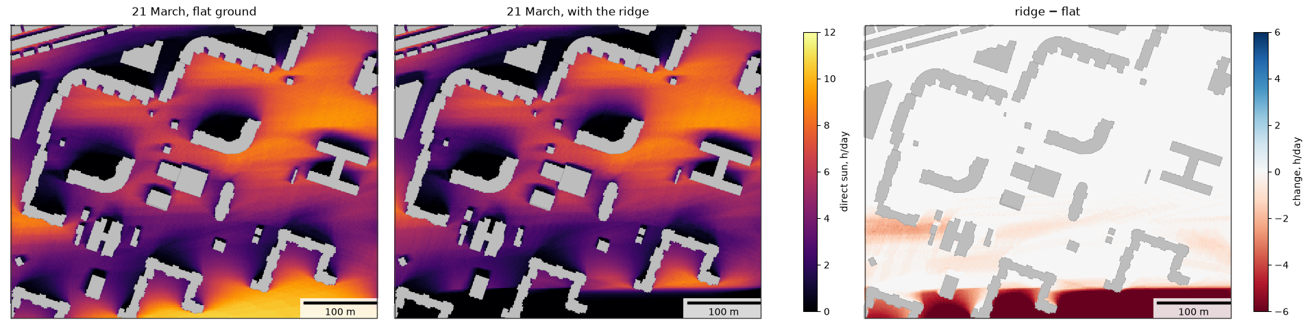
mean sun hours: flat 4.60 h, with the ridge 3.69 h; 11% of the open ground loses more than 1 h

Rasters on a web map and in GIS

Raster.explore shows the raster on a folium map with a colour bar, like GeoDataFrame.explore(); pass a map as the first argument to add the layer to it. Web maps draw images in Web Mercator, so the grid is resampled to a Mercator grid first and lines up with the base map; cells without a value are transparent. Raster.to_folium returns the bare image overlay, and Raster.to_geotiff(path) writes a GeoTIFF for QGIS or ArcGIS (requires rasterio).

hilly_r.explore(cmap="inferno", vmin=0, vmax=12, opacity=0.8, name="direct sun on 21 March, h")

Make this Notebook Trusted to load map: File -> Trust Notebook

5. Facades per floor

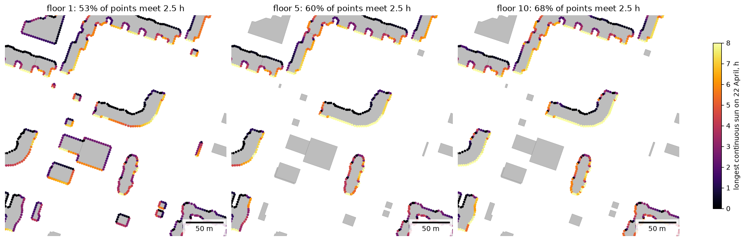
get_facade_insolation places points every spacing metres along the walls of the buildings intersecting area, on every floor at window_height above the floor level. The sun counts while it is in front of the facade and the ray towards it is clear. norm_hours adds meets_norm, the check of the longest continuous sunlit period.

The example uses 22 April and 2.5 h of continuous sun as the norm value; use the calculation day and the value of the norm that applies to the project (for Russia, SanPiN 1.2.3685-21).

target = shapely.box(344900, 6649950, 345150, 6650200)
facades = get_facade_insolation(scene, "2026-04-22", area=target, spacing=3, window_height=1.2, norm_hours=2.5, **HEIGHTS)
print(len(facades), "facade points on", facades["building"].nunique(), "buildings")
facades.drop(columns="geometry").head()

14945 facade points on 25 buildings

	building	floor	height	facade_azimuth	sun_hours	min_sun_hours	max_continuous_hours	meets_norm
0	95	1	1.2	291.080748	2.500000	2.500000	2.166667	False
1	95	2	4.2	291.080748	2.666667	2.666667	2.333333	False
2	95	3	7.2	291.080748	2.833333	2.833333	2.500000	True
3	95	4	10.2	291.080748	2.833333	2.833333	2.500000	True
4	95	5	13.2	291.080748	3.000000	3.000000	2.666667	True

by_floor = facades.groupby("floor").agg(
    points=("meets_norm", "size"), meets_norm=("meets_norm", "mean"), continuous_h=("max_continuous_hours", "median")
)
by_floor["meets_norm"] = (100 * by_floor["meets_norm"]).round(1)
by_floor.rename(columns={"meets_norm": "meets norm, %", "continuous_h": "median continuous sun, h"})

	points	meets norm, %	median continuous sun, h
floor
1	1238	53.0	2.500000
2	969	55.9	2.833333
3	949	58.0	3.000000
4	949	59.0	3.166667
5	949	60.1	3.333333
6	949	61.6	3.500000
7	949	62.7	3.666667
8	949	64.2	3.833333
9	949	66.3	4.000000
10	949	68.0	4.166667
11	949	70.5	4.333333
12	949	72.9	4.666667
13	949	77.3	4.833333
14	949	82.2	5.666667
15	509	83.5	6.000000
16	509	87.4	6.500000
17	83	63.9	6.500000
18	83	68.7	6.500000
19	83	85.5	6.500000
20	83	89.2	6.500000

from matplotlib import colors as mcolors

norm = mcolors.Normalize(0, 8)
x0, y0, x1, y1 = target.buffer(20).bounds
fig, axs = plt.subplots(1, 3, figsize=(15, 5), constrained_layout=True)
for ax, floor in zip(axs, [1, 5, 10]):
    sub = facades[facades["floor"] == floor]
    scene.plot(ax=ax, color="#bdbdbd", edgecolor="#8c8c8c", linewidth=0.3)
    sub.plot(ax=ax, column="max_continuous_hours", cmap="inferno", norm=norm, markersize=6)
    map_extent(ax, (x0, y0, x1, y1), bar=50, outline=False)
    ax.set_title(f"floor {floor}: {sub['meets_norm'].mean():.0%} of points meet 2.5 h")
fig.colorbar(plt.cm.ScalarMappable(norm=norm, cmap="inferno"), ax=axs, shrink=0.7,
             label="longest continuous sun on 22 April, h")
plt.show()

Buildings with the lowest share of facade points meeting the norm on the ground floor:

ground = facades[facades["floor"] == 1]
per_building = ground.groupby("building")["meets_norm"].agg(["size", "mean"]).rename(
    columns={"size": "points", "mean": "share meeting norm"}
)
per_building.sort_values("share meeting norm").head(5).round(2)

	points	share meeting norm
building
1274	59	0.22
102	95	0.37
408	20	0.40
2841	22	0.41
95	203	0.48

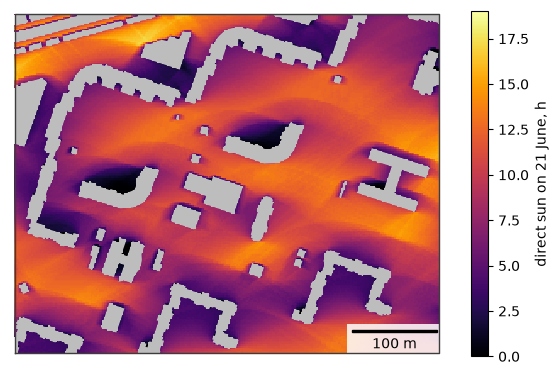
6. Your own area

Building footprints with heights or storeys and an area. The buildings around the area cast shadows into it, so pass them too. Raster.plot draws the raster, Raster.explore shows it on a web map with a colour bar and Raster.to_geotiff writes a GeoTIFF for GIS (requires rasterio).

my_buildings = buildings                                  # your footprints; HEIGHTS names the height columns
my_area = shapely.box(344750, 6649850, 345250, 6650250)   # your area, in the CRS of the buildings
my_scene = my_buildings[my_buildings.intersects(my_area.buffer(300))]

sun = rasterize(get_insolation(my_scene, "2026-06-21", area=my_area, grid_step=2, **HEIGHTS),
                "sun_hours")
fig, ax = plt.subplots(figsize=(7, 5.6))
gpd.GeoSeries([my_area]).plot(ax=ax, color="#bdbdbd", zorder=0)  # cells without a receiver lie under buildings
im = sun.plot(ax=ax, cmap="inferno", vmin=0, vmax=19)
my_scene.clip(my_area).plot(ax=ax, color="#bdbdbd", linewidth=0)
map_extent(ax, my_area.bounds)
fig.colorbar(im, ax=ax, shrink=0.8, label="direct sun on 21 June, h")
plt.show()
# sun.to_geotiff("my_sun_hours.tif")  # for GIS

sun.explore(cmap="inferno", vmin=0, vmax=19, name="direct sun on 21 June, h")

Make this Notebook Trusted to load map: File -> Trust Notebook

Limitations

Roofs are flat; balconies, loggias, window reveals and trees are not modelled, and only direct sunlight is counted. Values are multiples of time_step_min. See the insolation page for details.