Visibility Analysis
Visibility analysis estimates which buildings, barriers, or areas are visible from one or multiple observer points within a given distance. It is commonly used in studies of visual accessibility, urban perception, noise propagation, and urban form analysis.
The module provides a unified interface for visibility computation through the
objectnat.get_visibility()function, supporting both high-accuracy and fast approximate algorithms. The user can compute visibility from a single point or from a large batch of points in parallel.
Visibility Methods
Two algorithmic modes are available through the method parameter:
- Accurate method (``method=”accurate”``)
Performs detailed visibility computation based on obstacle boundaries, angular relations, and iterative polygon subtraction. This method captures narrow occlusions, corners, and complex geometry with high precision, making it ideal for urban micro-scale analysis.
- Simple method (``method=”simple”``)
Computes visibility using radial rays projected from the observer. It is significantly faster and suitable for large datasets, noise modelling, and regional-scale visibility studies.
Both methods are accessed via a single API:
- objectnat.get_visibility(point_from, obstacles, view_distance=None, method='accurate', *, resolution=32, parallel=False, max_workers=None)[source]
Compute visibility polygons for one or many observer points.
This is a high-level, batch interface to the visibility analysis:
Accepts a GeoDataFrame of observer points.
Reprojects points and obstacles to a locally estimated projected CRS (typically UTM) for distance-accurate calculations.
- For each point, computes a visibility polygon using either:
an accurate wall-based algorithm (
method="accurate"), ora simple ray-based approximation (
method="simple").
Supports per-point visibility radii via a dedicated column or a global
view_distancevalue.Optionally parallelizes computation across points using processes and can display a tqdm progress bar.
- Parameters:
point_from (
geopandas.GeoDataFrame) – GeoDataFrame with point geometries representing observer locations. Must have a valid CRS. Any additional attributes are preserved in the output.obstacles (
geopandas.GeoDataFrame) – GeoDataFrame with obstacle geometries in the same CRS aspoint_from. If empty orNone, no occlusion is applied and visibility is limited only by the viewing radius.view_distance (
float | None, optional) – Global viewing radius for all points (in units of the CRS). Used when the"visibility_distance"column is not present inpoint_from. IfNoneand the column is also missing, aValueErroris raised.method (
Literal[``”accurate”, ``"simple"], optional) –Visibility algorithm to use:
"accurate"– slower but more precise, based on obstacle boundaries and visibility wedges."simple"– faster approximation with radial rays and obstacle cutting.
resolution (
int, optional) – Resolution parameter for the simple method. Passed asquad_segstoPoint.buffer(); ignored whenmethod="accurate".parallel (
bool, optional) – IfTrue, compute visibility polygons for multiple points in parallel using processes. IfFalse, process points sequentially in the current process.max_workers (
int | None, optional) – Maximum number of worker processes whenparallel=True. IfNone, the default fromProcessPoolExecutoris used.
- Returns:
GeoDataFrame with the same index and attributes as
point_from, but with the geometry column replaced by visibility polygons. The result is returned in the original CRS ofpoint_from.- Return type:
gpd.GeoDataFrame
- Raises:
TypeError – If
point_fromis not a GeoDataFrame.ValueError – If
point_fromis empty, has no CRS, or neitherview_distancenor the"visibility_distance"column is provided.
Notes
If a column named
"visibility_distance"is present inpoint_from, its values are used as per-point view distances and theview_distanceargument is ignored.When
parallel=Trueandenable_tqdmis True in the global config, a progress bar is displayed usingtqdm.contrib.concurrent.process_mapduring parallel execution.
Differences between methods
method="accurate":Uses obstacle boundaries and angular visibility wedges. More precise, especially in dense environments and around corners, but slower.
method="simple":Uses radial rays and line splitting. Much faster and suitable for large batches or rough estimates, but may produce less detailed visibility shapes.
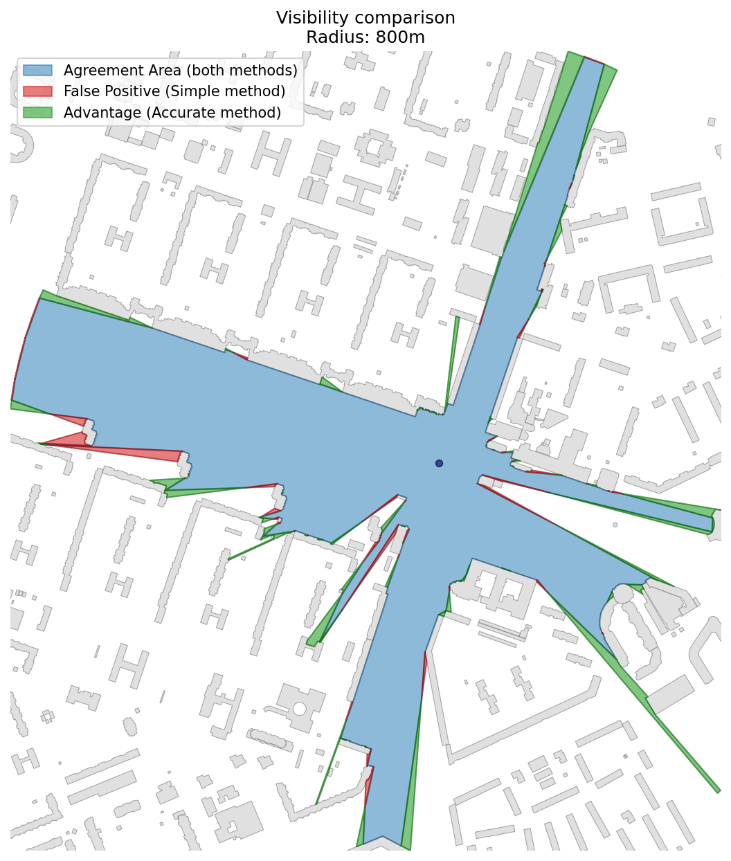
Comparison between accurate (boundary-based) and simple (ray-based) methods.
Catchment Visibility from Multiple Points
Performs visibility analysis for a dense grid of observer points, producing combined catchment visibility zones — areas showing where specific objects (e.g., landmarks, buildings) can be seen from.
Example of visibility polygons aggregated into visibility pools — zones most visible from multiple locations in an urban environment.